Time Series Forecasting
FEDOT allows you to automate machine learning pipeline design for time-series forecasting.
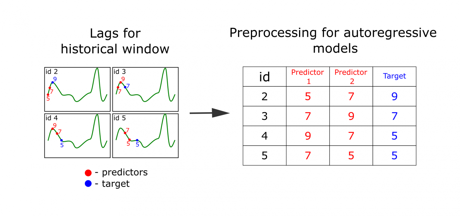
FEDOT extracts features using lagged transformation to apply regression methods for forecasting. Therefore not only models specific for time-series forecasting (such as ARIMA and AR) can be used but also any regression method (ridge, lasso, etc.).
Time-series specific preprocessing methods, like moving average smoothing or Gaussian smoothing are used as well.
Simple examples
You can find all available API parameters in Fedot reference.
Automated
Use FEDOT in automated mode to get pipeline with automatically composed architecture and tuned hyperparameters.
from fedot.api.main import Fedot
from fedot.core.data.data import InputData
from fedot.core.data.data_split import train_test_data_setup
from fedot.core.repository.tasks import Task, TaskTypesEnum, TsForecastingParams

# specify the task and the forecast length (required depth of forecast)
task = Task(TaskTypesEnum.ts_forecasting,
            TsForecastingParams(forecast_length=10))

# load data from csv
train_input = InputData.from_csv_time_series(task=task,
                                             file_path='time_series.csv',
                                             delimiter=',',
                                             target_column='value')
# split data for train and test
train_data, test_data = train_test_data_setup(train_input)

# init model for the time-series forecasting
model = Fedot(problem='ts_forecasting', task_params=task.task_params)

# run AutoML model design
pipeline = model.fit(train_data)
# plot obtained pipeline
pipeline.show()

# use model to obtain out-of-sample forecast with one step
forecast = model.forecast(test_data)
print(model.get_metrics(metric_names=['rmse', 'mae', 'mape'], target=test_data.target))

# plot forecasting result
model.plot_prediction()
Sample output:
Pipeline plot from the example:
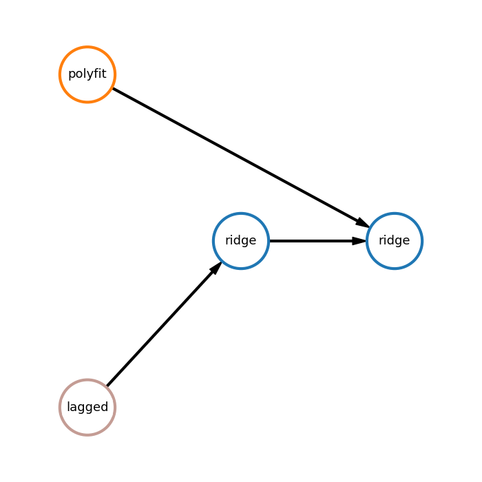
Here:
polyfit - polynomial interpolation,
lagged - lagged transformation,
ridge - ridge regression.
In the first branch polynomial interpolation is applied to obtain forecast. In the second branch lagged transformation is used to transform time-series into table data and then ridge is applied. Finally, another ridge model uses forecasts of two branches to generate final prediction.
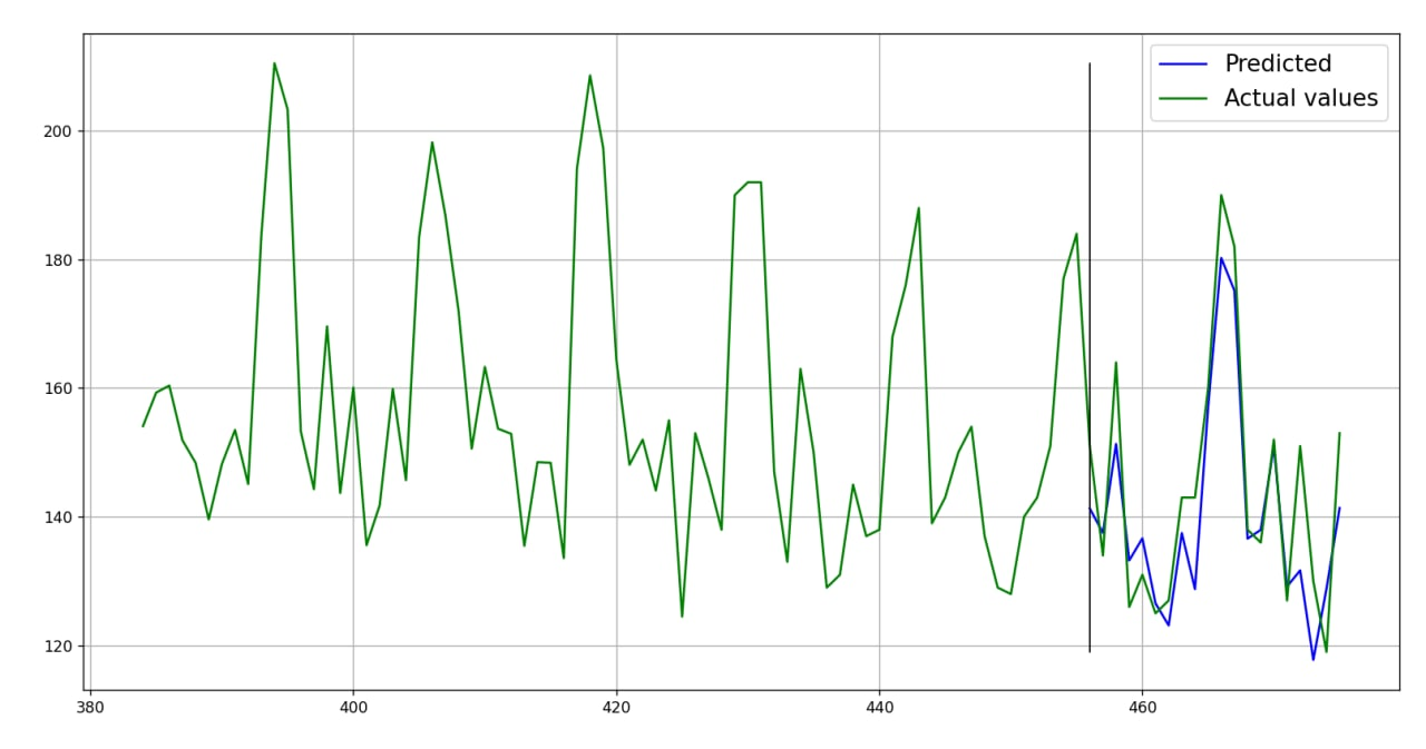
Obtained metrics:
{'rmse': 8.485, 'mae': 6.904, 'mape': 0.049}
Plot of the forecast:
Manual
Use FEDOT in manual mode to fit your own pipeline for time-series forecasting.
Examples of time-series pipelines can be found here.
See how to tune pipeline hyperparameters in Tuning of Hyperparameters.
from fedot.api.main import Fedot
from fedot.core.data.data import InputData
from fedot.core.data.data_split import train_test_data_setup
from fedot.core.pipelines.pipeline_builder import PipelineBuilder
from fedot.core.repository.tasks import Task, TaskTypesEnum, TsForecastingParams

# compose your own pipeline
pipeline = PipelineBuilder() \
    .add_sequence('lagged', 'ridge', branch_idx=0) \
    .add_sequence('glm', branch_idx=1).join_branches('ridge').build()

# specify the task and the forecast length (required depth of forecast)
task = Task(TaskTypesEnum.ts_forecasting,
            TsForecastingParams(forecast_length=10))

# load data from csv
train_input = InputData.from_csv_time_series(task=task,
                                             file_path='time_series.csv',
                                             delimiter=',',
                                             target_column='value')

# split data for train and test
train_data, test_data = train_test_data_setup(train_input)

# init model for the time-series forecasting
model = Fedot(problem='ts_forecasting', task_params=task.task_params)

# fit pipeline
model.fit(train_data, predefined_model=pipeline)

# use model to obtain one-step out-of-sample forecast
forecast = model.forecast(test_data)
print(model.get_metrics(metric_names=['rmse', 'mae', 'mape'], target=test_data.target))

# plot forecasting result
model.plot_prediction()
Sample output:
Pipeline plot from the example:
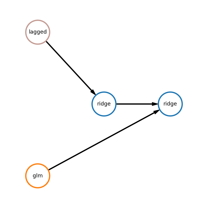
Here:
glm - generalized linear model,
lagged - lagged transformation,
ridge - ridge regression.
In the first branch lagged transformation is used to transform time-series into table data and then ridge is applied. In the second branch generalized linear model is applied to obtain forecast. Finally, another ridge model uses forecasts of two branches to generate final prediction.
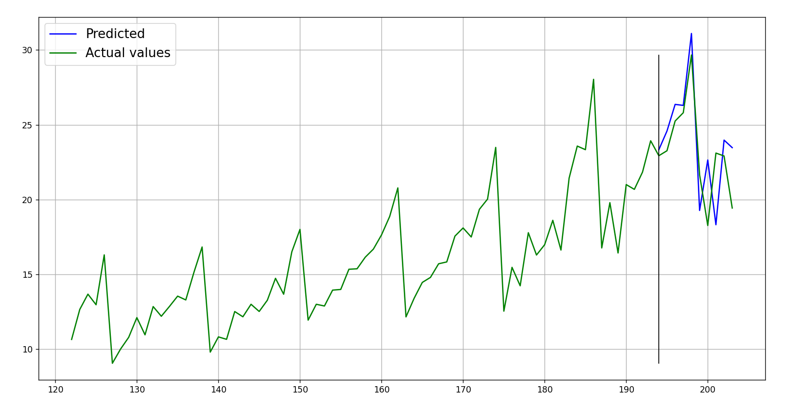
Obtained metric:
{'rmse': 2.659, 'mae': 2.142, 'mape': 0.100}
Plot of the forecast:
Time-series validation
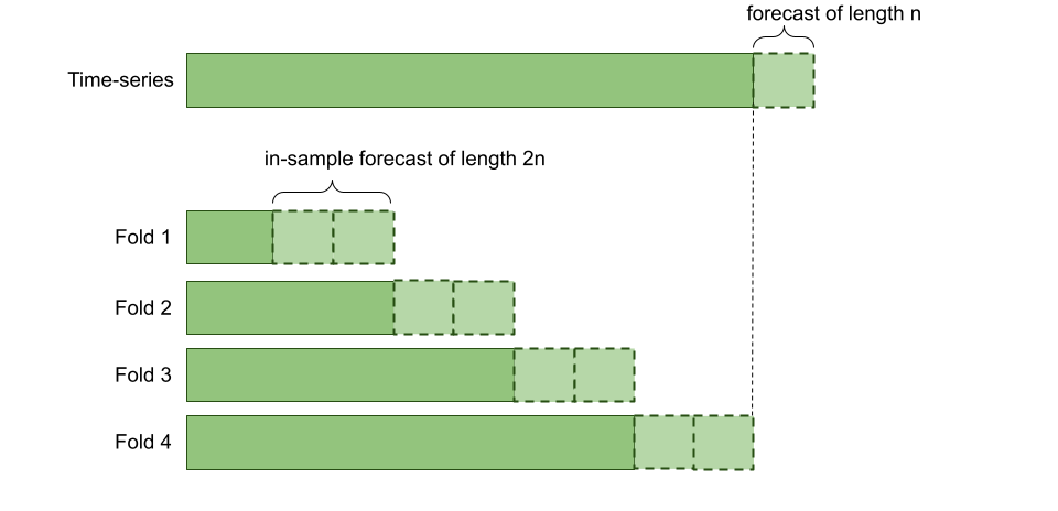
FEDOT uses in-sample forecasting for time-series validation.
While using FEDOT for forecasting you can set cv_folds parameter that sets number
of folds for cross validation of a time-series.
The size of validation sample in each fold is almost the maximum possible size and multiple of forecast_length.
Train test split
To split InputData use train_test_data_setup method.
split_ratio and shuffle, and stratify are ignored for time-series forecasting.
- fedot.core.data.data_split.train_test_data_setup(data, split_ratio=0.8, shuffle=False, shuffle_flag=False, stratify=True, random_seed=42, validation_blocks=None)[source]
Function for train and test split for both InputData and MultiModalData
- Parameters
data (Union[InputData, MultiModalData]) – InputData object to split
split_ratio (float) – share of train data between 0 and 1
shuffle (bool) – is data needed to be shuffled or not
shuffle_flag (bool) – same is shuffle, use for backward compatibility
stratify (bool) – make stratified sample or not
random_seed (int) – random_seed for shuffle
validation_blocks (Optional[int]) – validation blocks are used for test
- Returns
data for train, data for validation
- Return type
Tuple[Union[InputData, MultiModalData], Union[InputData, MultiModalData]]
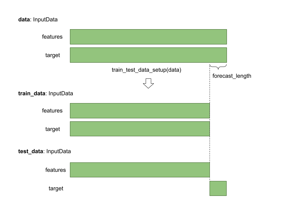
The method uses forecast_length specified in the data.task.
train_data, test_data = train_test_data_setup(train_input)
This approach can be used to
obtain `test_data` for out-of-sample forecast after training a model on the `train_data`.
The resulting split:
train_data.features = data.features[:-forecast_length]train_data.target = data.target[:-forecast_length]test_data.features = data.features[:-forecast_length]train_data.target = data.target[-forecast_length:]
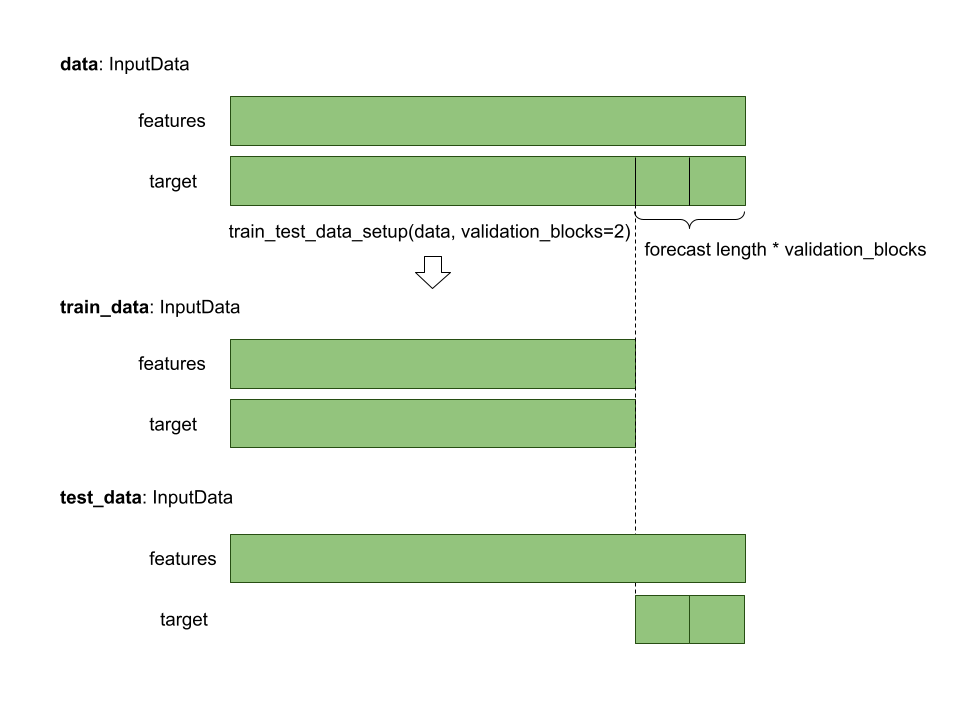
train_data, test_data = train_test_data_setup(train_input, validation_blocks=3)
If you pass keyword argument validation_blocks train data will be prepared for in-sample
validation with validation_blocks number of steps. In these case:
train_data.features = data.features[:-forecast_length * validation_blocks]train_data.target = data.target[:-forecast_length * validation_blocks]test_data.features = data.featurestrain_data.target = data.target[-forecast_length * validation_blocks:]
Prediction
There are two approaches to time-series forecasting: in-sample and out-of-sample. For example, our trained model forecasts 10 values ahead and our training sample length is 100. With in-sample forecast we will predict 10 last values of our training sample using 90 first values as prehistory. With out-of-sample we will predict 10 future values of the training sample using the whole sample of 100 values as prehistory.
To obtain forecast with length exceeding the forecast length (depth) model was trained for, we use iterative prediction. For example, our trained model forecasts 10 values ahead, but we want to forecast 20 values. With out-of-sample approach we would predict 10 values and then use those values to forecast another 10 values. But with in-sample approach we forecast already known parts of time-series. And after forecasting first 10 values we would use real values from time-series to forecast next 10 values.
You can use two methods for time-series forecasting: Fedot.predict - in-sample forecast, Fedot.forecast -
out-of-sample forecast.
In-sample forecast
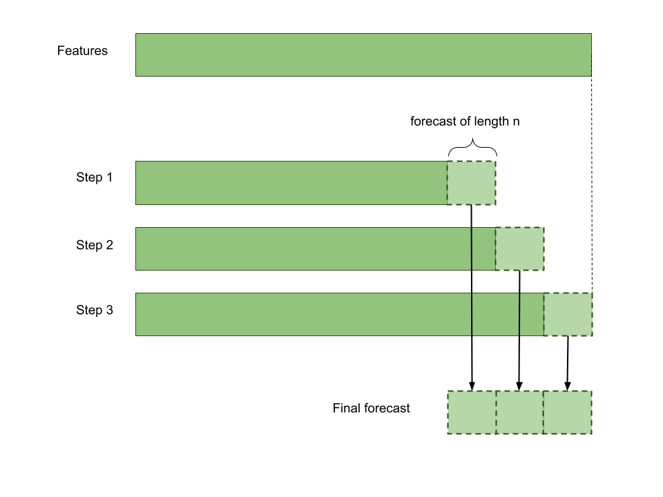
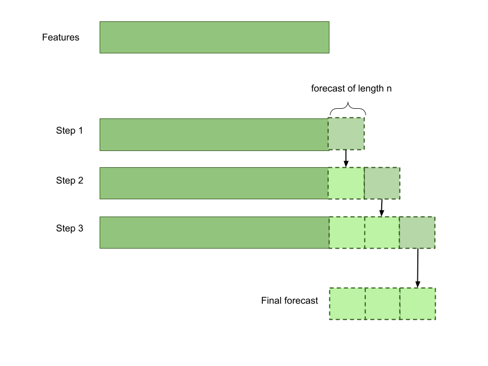
Fedot.predict allows you to obtain iterative in-sample forecast with depth of forecast_length * validation_blocks.
Method uses forecast_length specified in the task parameters. This method uses features as sample and gets forecast in the way
described in the picture (validation_blocks=3).
Example of in-sample forecast.
from fedot.api.main import Fedot
from fedot.core.data.data import InputData
from fedot.core.data.data_split import train_test_data_setup
from fedot.core.repository.tasks import Task, TaskTypesEnum, TsForecastingParams

# set task type and forecast length
task = Task(TaskTypesEnum.ts_forecasting,
            TsForecastingParams(forecast_length=10))

# load data from csv
train_input = InputData.from_csv_time_series(file_path='time_series.csv',
                                             task=task,
                                             target_column='value')

# split data for in-sample forecast
train_data, test_data = train_test_data_setup(train_input, validation_blocks=3)

# init model for the time-series forecasting
model = Fedot(problem='ts_forecasting', task_params=task.task_params, cv_folds=2)

# run AutoML model design
pipeline = model.fit(train_data)

# use model to obtain three-step in-sample forecast
in_sample_forecast = model.predict(test_data, validation_blocks=3)

# get metrics for the prediction
print('Metrics for three-step in-sample forecast: ',
      model.get_metrics(metric_names=['rmse', 'mae', 'mape'], validation_blocks=3))

# plot forecasting result
model.plot_prediction()
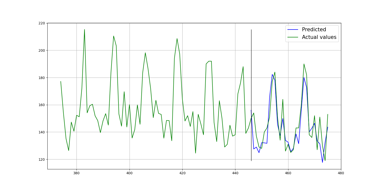
Plot of the forecast:
Another example of in-sample forecast.
...
# split data for in-sample forecast
train_data, test_data = train_test_data_setup(train_input, validation_blocks=2)

# init model for the time-series forecasting
model = Fedot(problem='ts_forecasting', task_params=task.task_params,
              cv_folds=2)

# run AutoML model design
pipeline = model.fit(train_data)

# use model to obtain two-step in-sample forecast while using 3 validation blocks for fit
in_sample_forecast = model.predict(test_data, validation_blocks=2)

# get metrics for the prediction
print('Metrics for two-step in-sample forecast: ',
      model.get_metrics(metric_names=['rmse', 'mae', 'mape'], validation_blocks=2))

# plot forecasting result
model.plot_prediction()
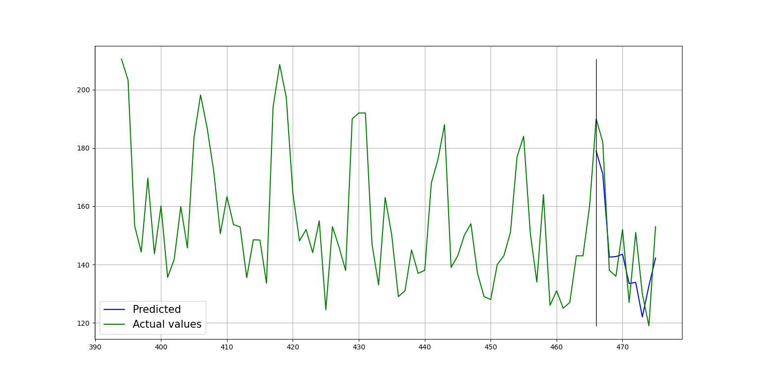
Plot of the forecast:
Out-of-sample forecast
Fedot.forecast can be used to obtain out-of-sample forecast with custom forecast horizon. If
horizon > forecast_length forecast is obtained iteratively using previously forecasted values to
predict next ones at each step. If horizon < forecast_length forecast is cutted according to the horison.
By default horizon = forecast_length.
Example of forecast with default horizon.
from fedot.api.main import Fedot
from fedot.core.data.data import InputData
from fedot.core.data.data_split import train_test_data_setup
from fedot.core.repository.tasks import Task, TaskTypesEnum, TsForecastingParams

# set task type and forecast length
task = Task(TaskTypesEnum.ts_forecasting,
            TsForecastingParams(forecast_length=10))

# load data from csv
train_input = InputData.from_csv_time_series(file_path='time_series.csv',
                                             task=task,
                                             target_column='value')

# split data for out-of-sample forecast
train_data, test_data = train_test_data_setup(train_input)

# init model for the time-series forecasting
model = Fedot(problem='ts_forecasting', task_params=task.task_params, cv_folds=2)

# run AutoML model design
pipeline = model.fit(train_data)

# use model to obtain one-step out-of-sample forecast
out_of_sample_forecast = model.forecast(test_data)

# get metrics for the prediction
print('Metrics for out-of-sample forecast: ',
      model.get_metrics(metric_names=['rmse', 'mae', 'mape']))

# plot forecasting result
model.plot_prediction()
Plot of the forecast:
Example of forecast with horizon > forecast_length.
...
# split data for out-of-sample forecast
train_data, test_data = train_test_data_setup(train_input)

# init model for the time-series forecasting
model = Fedot(problem='ts_forecasting', task_params=task.task_params, cv_folds=2)

# run AutoML model design
pipeline = model.fit(train_data)

# use model to obtain out-of-sample forecast with horizon = 25 (> forecast_length)
in_sample_forecast = model.forecast(test_data, horizon=25)

# plot forecasting result
model.plot_prediction()
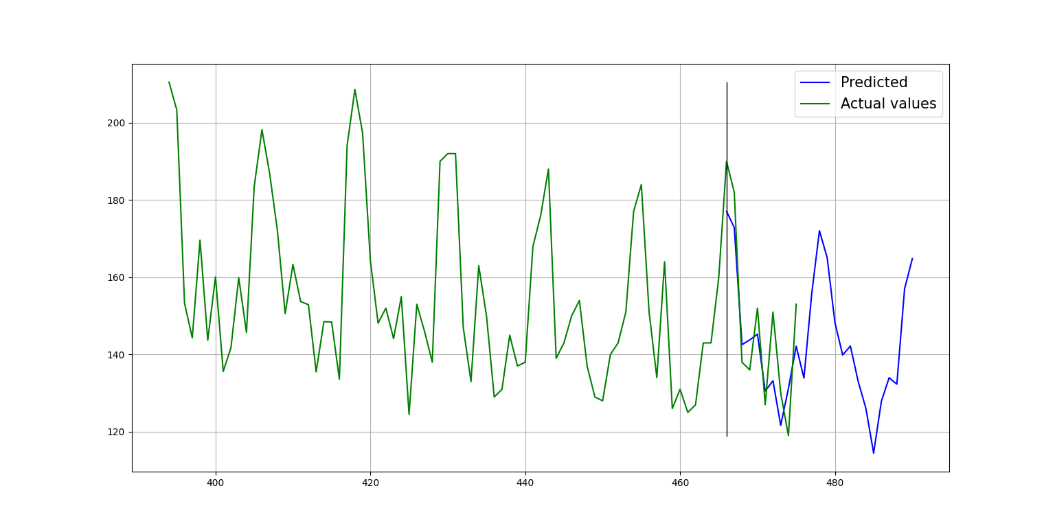
Plot of the forecast:
Multivariate time-series forecasting
FEDOT allows you to forecast multivariate time-series.
Use multi time-series approach to forecast one time-series, while model was trained on the number of time-series of the same variable as target. At first, lagged transformation is applied to transform all of the time-series to table data then regression models are used. (Using several time-series allows you to expand training sample - after lagged transformation you get more train/target pairs).
from fedot.api.main import Fedot
from fedot.core.data.data import InputData
from fedot.core.data.data_split import train_test_data_setup
from fedot.core.repository.tasks import Task, TaskTypesEnum, TsForecastingParams

# name of the column with target time-series
target = 'col_3'

# set task type and forecast length
task = Task(TaskTypesEnum.ts_forecasting,
            TsForecastingParams(forecast_length=20)) # forecast_length - required depth of forecast

# load data from csv
data = InputData.from_csv_multi_time_series(
        file_path='time_series.csv',
        task=task,
        target_column=target,
        columns_to_use=['col_1', 'col_2', 'col_3', ..., 'col_n'])

# split data for in-sample forecast
train_data, test_data = train_test_data_setup(data, validation_blocks=2)

# init model for the time-series forecasting
model = Fedot(problem='ts_forecasting',
              task_params=task.task_params,
              timeout=5,
              n_jobs=-1,
              cv_folds=2)

# run AutoML model design
pipeline = model.fit(train_data)
# plot obtained pipeline
pipeline.show()

# use model to obtain two-step in-sample forecast
forecast = model.predict(test_data, validation_blocks=2)
print(model.get_metrics(metric_names=['rmse', 'mae', 'mape'],
                        target=test_data.target, validation_blocks=2))
Sample output:
Pipeline plot from the example:
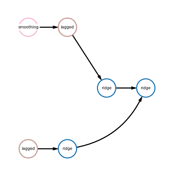
Here:
smoothing - rolling mean,
lagged - lagged transformation,
ridge - ridge regression.
In the first branch time-series is transformed using rolling mean, lagged transformation is used to transform time-series into table data and then ridge is applied. In the second branch only lagged transformation is applied before using ridge. Finally, another ridge model uses forecasts of two branches to generate final prediction.
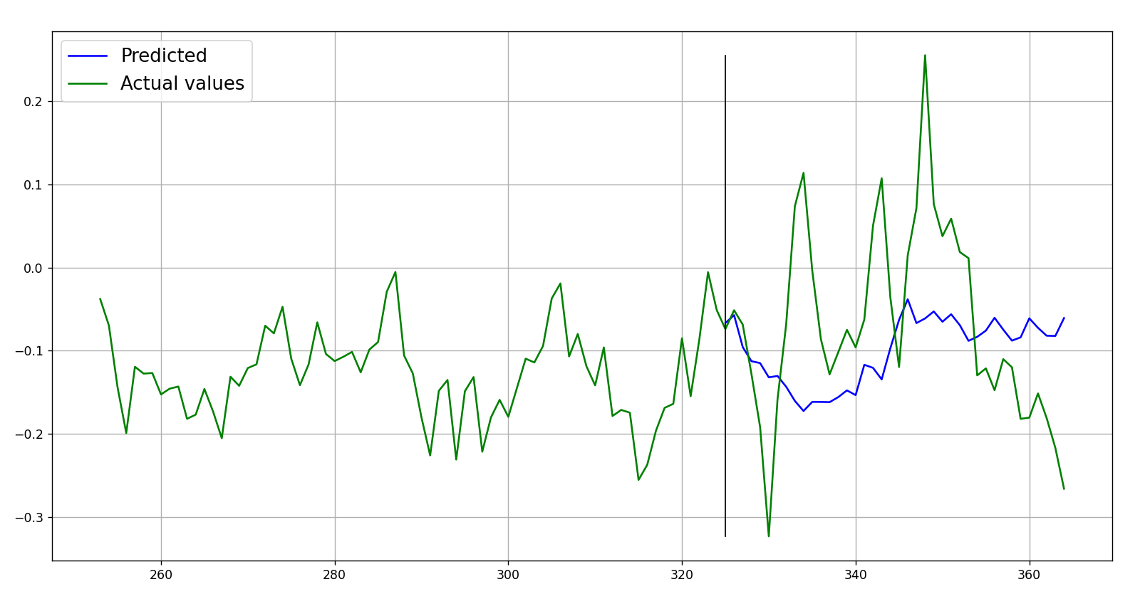
Obtained metric:
{'rmse': 0.105, 'mae': 0.087, 'mape': 0.469}
Plot of the forecast:
Use multimodal approach to forecast a time-series using several other time-series. In this case for every time-series a data sourse node will be created.
import numpy as np
import pandas as pd

from fedot.api.main import Fedot
from fedot.core.repository.tasks import TsForecastingParams
from fedot.core.utils import fedot_project_root

forecast_length = 10

# load data from csv
df_train = pd.read_csv('data_train.csv'))

# get time-series
ws_history = np.ravel(np.array(df_train['wind_speed']))[:200]
ssh_history = np.ravel(np.array(df_train['sea_height']))[:200]

# use dict as input data
historical_data = {
    'ws': ws_history,  # additional variable
    'ssh': ssh_history,  # target variable
}

# init model for the time-series forecasting
fedot = Fedot(problem='ts_forecasting',
              task_params=TsForecastingParams(forecast_length=forecast_length),
              timeout=10)

# run AutoML model design
pipeline = fedot.fit(features=historical_data,
                     target=ssh_history)  # specify target time-series

# get in-sample forecast
fedot.predict(historical_data)

# get metrics
metric = fedot.get_metrics(ssh_history[-forecast_length:])

pipeline.show()
fedot.plot_prediction(target='ssh')
Sample output:
Pipeline plot from the example:
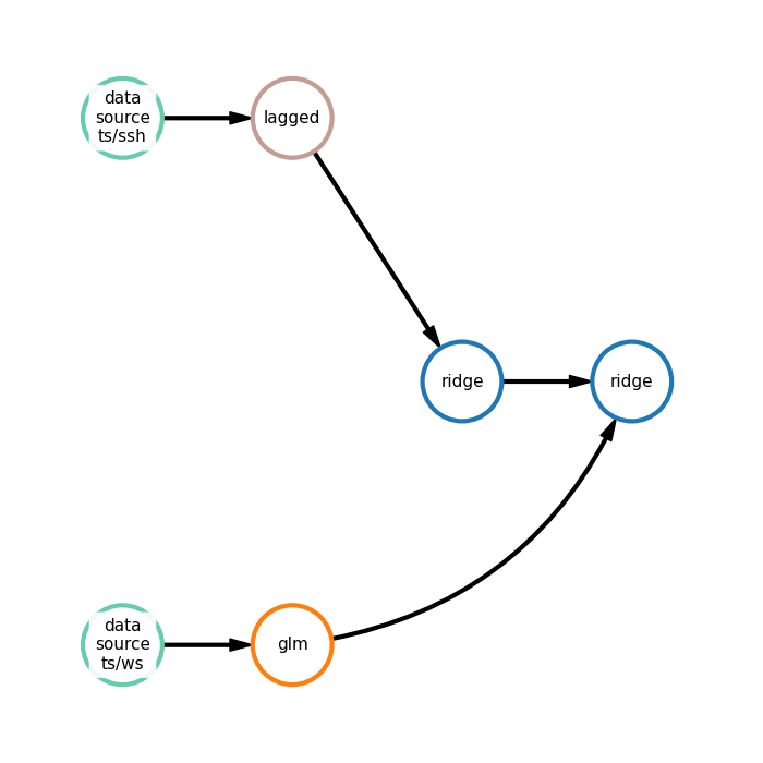
Here:
glm - generalized linear model,
lagged - lagged transformation,
ridge - ridge regression,
data_source_ts/ws - data input node for ws time-series,
data_source_ts/ssh - data input node for ssh time-series
In the first branch time-series is transformed using lagged transformation and then ridge is applied. In the second branch only generalized linear model is applied. Finally, another ridge model uses forecasts of two branches to generate final prediction.
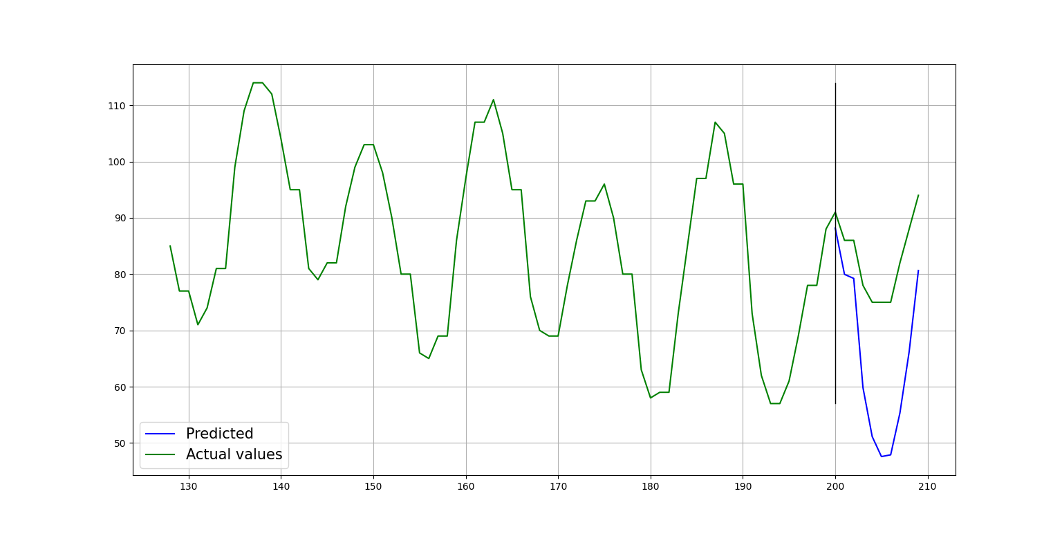
Obtained metric:
{'rmse': 11.578, 'mae': 10.400}
Plot of the forecast:
Lagged transformation
To extract features FEDOT uses lagged transformation (windowing method) which allows to represent time-series as trajectory matrix and apply regression methods for forecasting.
Examples
Simple
Advanced
Cases